SN2015M
Things that go Bang in the Night
Project Aims
In May 2015 a type Ia supernova (SN2015M) was discovered in the Coma cluster of galaxies. CCD images of this supernova were taken using Durham’s DRACO2 telescope. The project will fully process these images in order to determine the characteristics of SN2015M and undertake some basic scientific analysis. This will include constructing a calibrated V-band light curve, measuring the peak brightness and decline rate, deriving the various characteristics of this supernova, comparing and contrasting SN2015M to other SNIa including those previously seen in the Coma cluster like SN2010ai, estimating the Hubble constant and linking the results with other recent SNIa studies.
Key Outcomes
- an understanding of Hubble’s law and the expansion of the universe
- a knowledge of how the distance to Type Ia supernovae can be determined including the zero-point calibration
- measurement of the light curve of a recent SNIa, i.e. SN2015M, via aperture photometry
- analysis of the light curve including a distance measurement of SN2015M
- an estimate (plus uncertainty) of the Hubble constant from the analysis of SN2015M
- construction of a report describing the study carried out
Introduction
Supernovae are exploding stars which at peak brightness can be ∼1010 times the luminosity of the Sun. Their high intrinsic luminosity means that they can be observed at great distances in the universe.
In mid-May 2015, a supernova (SN2015M = PS15apc) in the Coma cluster of galaxies was independently discovered by several observers ( CBET4123 ) including Nakano, S (Sumoto, Japan), Itagaki, K (Teppo-cho, Yamagata, Japan) and Lucey, J R (Durham, UK).
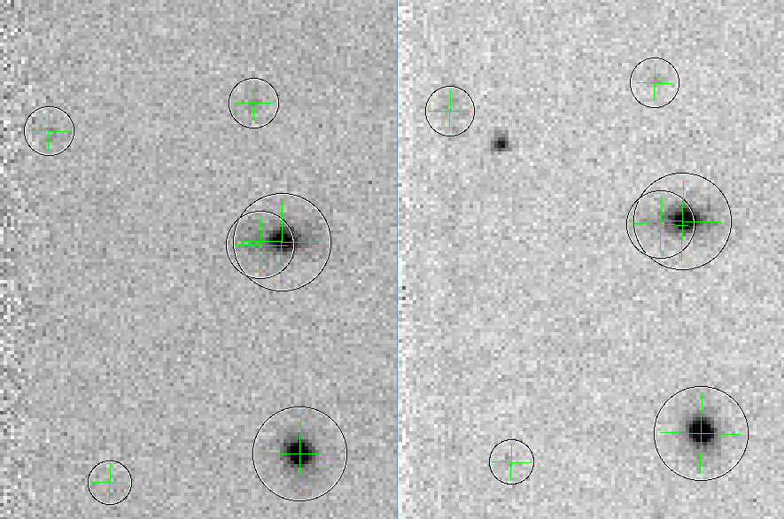
The figure below shows the before/after comparison images of SN2015M taken at Durham; on the left is an archive image and on the right is the discovery image taken on 2015 May 12 at 22:00 UTC. The overlayed circles/crosses denote the previously catalogued Coma cluster galaxies and foreground stars at this location in the sky. SN2015M is readily apparent on the right-hand image.
The Coma cluster (Abell 1656, NED link) lies at a distance of about 100 Mpc and is one of the richest dense grouping of galaxies in the nearby universe. SN2015M was “hostless” in the sense it was not directly near any of the bright Coma cluster galaxies. The progenitor of SN2015M may have been a free-floating intra-cluster star which was torn from its host galaxy by the tidal forces in the dense cluster environment. A previous hostless Ia supernova in the Coma cluster was SN2010ai.
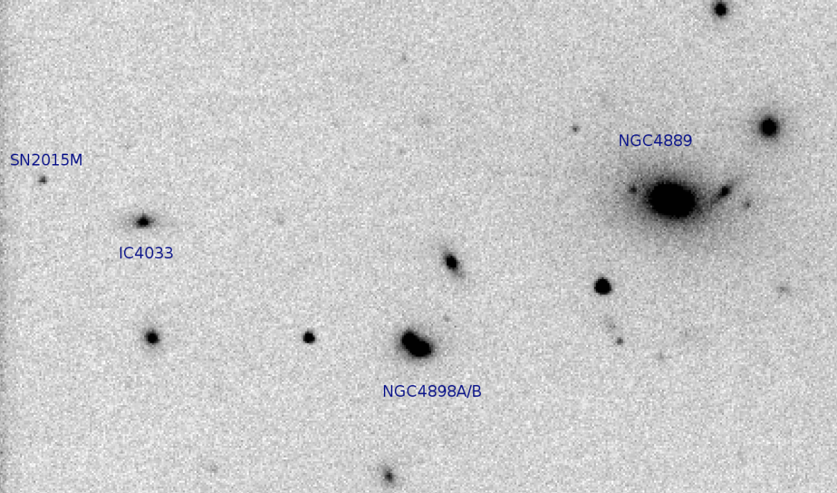
Below is a wider area image showing the location of SN2015M with respect to Coma cluster galaxies NGC4889, NGC4898A/B and IC4033.
By analysing the light curve of SN2015M the distance to this supernova (and the Coma cluster) can determined which then can be used to measure of the Hubble constant.
Background to Magnitudes: Apparent and Absolute
In astronomy the term luminosity refers to the energy emitted by a source per unit time. The term flux refers to the energy per unit area per unit time received from a source by an observer at a distance. The flux f received from a source of luminosity L at a distance d is
f = L / ( 4 π d2 ) hence L = 4 π d2 f ; i.e. the inverse square law .
Apparent magnitude is the measure of the observed flux of a celestial object as seen from the Earth. The ancient Greek astronomers divided the stars visible to the naked eye into six magnitude groups. The first magnitude stars were the brightest, whilst the faintest stars visible to the naked eye were of 6th magnitude. When, in the 19th century, a quantitative system was developed it was made to agree approximately with the old system. This led to the defining equationm = constant − 2.5 log10 ( f )
where m is the apparent magnitude, f is the observed flux and the constant defines the zero-point of the magnitude scale.
In practice, the apparent magnitude of a object X is measured by reference to a standard star of known apparent magnitude, i.e.mX = mSTD − 2.5 log10 ( fX / fSTD ) .
Measure fX and fSTD, take mSTD from a catalogue and hence determine mX.
There are magnitude systems for different wavebands, i.e. the flux is measured in a restricted range of wavelengths, e.g. the visual band (V-band) λ centre = 550 nm, Δλ = 100 nm, the blue band (B-band) λ centre = 450 nm, Δλ = 100 nm.
The absolute magnitude M of a star is the apparent magnitude it would have if it were seen at a distance of 10 parsecs. As the observed flux of an object is diluted by the inverse square law, m and M are related via,m − M = 5 log10d − 5
where d is the distance in units of parsecs (one parsec = 206265 AU = 3.0857 × 10¹⁶ m ). m − M is called the distance modulus.
In astronomy the term standard candle is used for an object that has a known intrinsic brightness, i.e. M is known. The distance of the object can then be calculated by measuring m.
Background to Type Ia Supernovae
A supernova is the explosion of a star. Several distinct classes of supernova have been recognised and given types, i.e. Ia, Ib, Ic, II-P, II-L, IIn and IIb. Type Ia Supernova (SNIa) are characterized by the lack of hydrogen in their spectrum. They probably result from a carbon-oxygen white dwarf (WD) in a close binary system accreting mass above the Chandrasekhar limit (1.4 solar masses). The nature of the donor star is still disputed: Single Degenerate (WD + Main sequence or red giant or He star companion) vs Double Degenerate (WD + WD merger) scenarios or both.
Optical spectra of SN2015M taken by Mazzali et al. (2015) on May 13 and May 15 “shows good matches with a pre-maximum 1991T-like type-Ia supernovae, showing high ionization lines of Fe II and Fe III. The redshift estimated from the spectral fitting of the supernova spectra is roughly consistent with the Coma cluster redshift”.
As well as using spectral information, the light curve of a supernova, i.e. how its brightness changes as a function of time, can also be used to identify the supernova type. SNIa have a distinct light curve shape. The distance to a SNIa can be determined from the light curve.
SNIa are standard candles (after a correction for the “stretch factor”; luminous SNIa fade slowly and less luminous SNIa fade fast) and can be used to measure the distance to their parent galaxy (or galaxy cluster) with a precision of 10% or better.
Details on the “stretch factor”, i.e. the “luminosity-decline rate relation” first found by Phillips (1993) are described on Swinburne’s web page on SNIa light curves.
In order to calibrate the absolute magnitude of SNIa light curves independent distances to galaxies that have hosted a SNIa are used and extensive observing programmes have been undertaken just for this task, e.g. see SNIa HST Calibration Program ( Sandage et al. 2006 ) and the SH0ES project ( Hoffmann et al. 2016 ).
Background to Hubble’s law
Hubble’s law describes the observed linear relation between velocity and distance that is found for galaxies (and galaxy clusters like Coma), i.e.
v = H0d
where v is the recession velocity in km/s, d is the distance in Mpc and H0 is the Hubble constant in km/s/Mpc. For studies in the nearby universe we assume v = czCMB, where c is the velocity of light and zCMB is the redshift. The CMB subscript refers to z being measured in the local Cosmic Microwave Background rest frame; see this NASA NED page for more details. We use the term “Hubble flow” to describe the “motion” of galaxies due solely to the expansion of the Universe.
The Coma cluster has a mean czCMB of 7200 +/− 100 km/s. Apparent magnitude (m) measurements of SN2015M with an adopted absolute magnitude (M) enable the distance of SN2015M (and the Coma cluster) to be determined via the distance modulus equation. The derived distance from this equation, i.e.d = 10 ( (m − M) + 5) / 5
will allow a measurement of the Hubble constant to be made.
If the Hubble constant is 72 km/s/Mpc then the expected distance to the Coma cluster would be 7200/72 = 100 Mpc, i.e. a distance modulus of 35. Using the IR Surface Brightness Fluctuation method (Jensen et al. 2015) measure a Coma cluster distance of 96 +/− 5 Mpc.
Project Notes and Questions
The key stages of the project will include:
- review of SNIa as standard candles and the extragalactic distance scale, e.g. how are SNIa made standard candles?; how is the absolute magnitude of SNIa determined?; what are current best estimates for this?
- review of SN2015M and reported measurements, e.g. are there any independent photometry measurements that could be used in the project?
- photometric measurements from the Durham CCD image data, choice of aperture sizes and calibration stars
- construction of the V-band light curve and comparsion with other SNIa light curves; from the light curve alone is SN2015M a Type Ia supernova?; how does SN2015M compare to previously observed supernovae in the core of the Coma cluster, particularly SN2010ai?; how similar is SN2015M’s light curve to that of SN1991T ?
- determination of the V-band peak brightness and a rough estimate of the stretch factor, Δm15(B); what are the uncertainties on these parameters?
- derive a distance to the Coma cluster. Compare and contrast this to other independent measurements of Coma’s distance including a distance to a previous hostless Ia supernova SN2010ai in Coma.
- derive a value of the Hubble constant with an uncertainty. Compare and contrast to independent measurements.
The DRACO2 CCD Image Data
The SN2015M observations were made with DRACO2 which is a 14-inch Meade LX200 telescope on the roof of the Physics Department. DRACO2 has a QSI 683ws CCD with a filter wheel (B, V, r). The CCD field-of-view is 18 × 13 arcmin and the pixel scale is 0.99 arcsec per pixel (with 3×3 binning). The list of observations made can be found in the DRACO2 2015 observing logs. The first V-band observations were made on 2015 May 16 and the last observation was made on 2015 June 18. Select suitable/best images for your analysis, i.e. V-band and the smallest PSF FWHM.
At the time of the observations a preliminary un-calibrated V-band light curve was constructed, i.e.
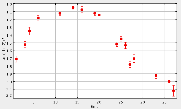
The x-axis is the time in days from the first observation. The y-axis is the supernova brightness, expressed in units of magnitudes, relative to two reference stars; a photometric zero-point calibration has not been applied so the y-axis zero-point is arbitrary.
Data Reduction Steps for the Photometric Measurements
The data analysis will be carried out on a set of linux ( Fedora ) workstations using the GAIA image display tool which provides a fast and simple interactive way to carry out aperture photometry of objects on astronomical images.The typical commands needed to process the CCD images would be:
 >> mkdir 15_05_16V                                          # create a work directory for the processing
 >> cd 15_05_16V                                             # move to that directory
 >> cp -p /mnt/archive/draco2/2015/15_05_16/d0070.fits .     # copy image d0070.fits to the current directory
 >> ls -lrt                                                  # check that the image has been copied
 >> gaia d0070.fits                                          # displays image d0070.fits with GAIA
Details on how to undertake aperture photometry are given on GAIA’s Aperture Photometry Toolbox web page. By default the magnitude zero-point is set to 50.00 and an instrumental magnitude is calculated via
magnitude = 50.0 − 2.5 log10 (flux)
where the flux is the background subtracted counts in the chosen circular aperture. For further background see the Astrolab page on basic photometry which has details on the choice of aperture radius. Ensure that the same aperture radius is used for all the measurements made for an image. It is recommended to simply record your basic measurements in instrumental magnitudes.
An uncertainty on the instrumental magnitude measurement is provided by GAIA. This approximately follows the formal way to estimate uncertainties as given in John Simonetti’s Measuring the Signal-to-Noise Ratio (S/N) of the CCD Image of a Star. This
The zero-point of the magnitude scale can be set by reference to a set of carefully selected calibration stars using the Pan-STARRS1 g- and r-band photometry via the bandpass transformation
B = 0.213 + gPS1 + 0.587 ( gPS1 − rPS1 )
V = 0.006 + gPS1 − 0.525 ( gPS1 − rPS1 )
(see Table 6 in Tonry et al. 2012). Check that the differences in the magnitudes of your calibration stars are constant within the uncertainties. Ensure that only stars, i.e. point sources, are used for the calibration as galaxies will give a bias as they are extended sources.
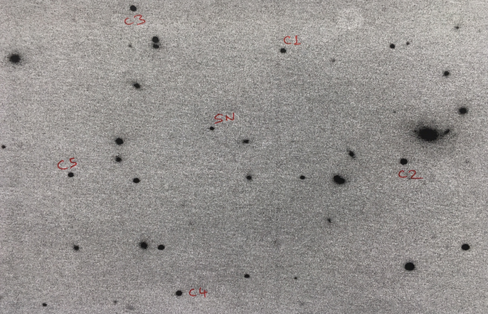
Possible calibration stars to used are:
# number  RA      Dec      g_PS1 g_err   r_PS1 r_err            B       V
   c1   195.1020 28.0135  15.371 0.007  15.025 0.003    -->   15.787  15.195
   c2   195.0445 27.9645  14.334 0.003  13.479 0.001    -->   15.049  13.891
   c3   195.1720 28.0310  14.864 0.002  14.532 0.006    -->   15.272  14.696
   c4   195.1486 27.9022  14.565 0.004  13.972 0.007    -->   15.126  14.260
   c5   195.2007 27.9557  15.042 0.007  14.675 0.003    -->   15.470  14.855
What is the likely systematic zero-point uncertainty on the photometric measurements?
In GAIA use the default magnitude zero-point, i.e. 50, and then difference the values returned to derive a calibrated magnitude for the supernova, i.e.
mag(supernova) = mag(supernova)’ − 0.5 [ mag(c1)’ + mag(c2)’ ] + 0.5 [ mag(c1) + mag(c2) ]
where mag(supernova)’, mag(c1)’ and mag(c2)’ are the instrumental magnitudes from GAIA, and mag(c1) and mag(c2) are the catalogued magnitudes for the 1st calibration star and the 2nd calibration star as determined by PS1. The background for this procedure is given here.
Use Modified Julian Day (MJD) to record the date/time of an observation. The MJD is defined as
MJD = JD – 2400000.5
where JD is the Julian Day. Start of the JD count is from 0 at 12 noon 1 JAN 4712 (4713 BC). The MJD can be found in the image fits header.
In order to reduce the error on the measured magnitudes a set of images can be averaged. We use the routines provided by Peter Draper’s CCDPACK software package to stack, i.e. register and average, a set of images via csh script. The typical commands needed to stack the CCD images would be:
 >> mkdir 15_05_16V                                          # create a work directory for the processing
 >> cd 15_05_16V                                             # move to that directory
 >> python /mnt/64bin/dfstack.py draco2 15_05_19 30 62       # average (stack) the "d" images in directory
 >> gaia amosaic.fits                                        # display the averaged image in GAIA
Note: the special procedure needed to estimate the photometry uncertainties correctly for the stacked images, i.e. set the “Measurement errors use:” to “sky variance”. See the section on Stacking Images webpage on Calculation of Photometric Errors in Stack Images.
Are your final statistical photometric errors reasonable?
Light Curve Construction and Distance Determination
Construct your light curve for SN2015M, i.e. plot MJD vs V-band apparent magnitude.
How does your light curve for SN2015M compare to a “standard” Ia light curve ?
Estimate the stretch factor and likely absolute magnitude for SN2015M.
Estimate the distance modulus to SN2015M.
Use SN(oo)Py to derive a more precise value for the distance modulus. Assume that the “host galaxy” has no internal extinction by setting EB-V = 0.00, i.e. in SN(oo)py fit the light curve with s.fit(EBVhost=0.0); this is a reasonable assumption as the supernova is hostless. Using an “arbitrary” photometric zero-point, results of SN(oo)Py are shown in the figure below; “arbitrary” = make the answer approximately correct.
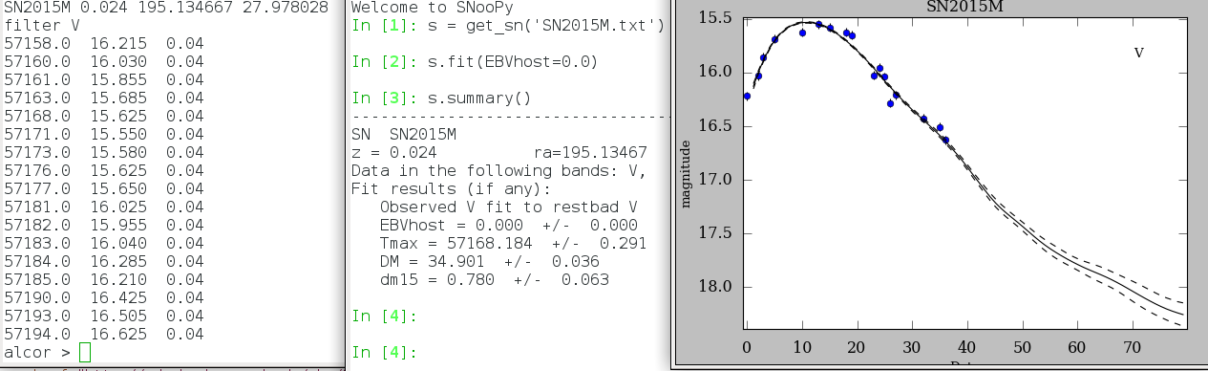
How does SN(oo)Py set the photometry zero-point of the SNIa light curve templates, i.e. the absolute magitude scale?
Is any correction included for the foreground galactic extinction, i.e. that from the Milky Way? What is the total error budget?
A previous hostless Ia supernova in the Coma cluster was SN2010ai. Light curve data is available from Hicken et al 2012. Use this literature data to derive an independent distance to the Coma cluster using SN(oo)Py.
Discussion
Derive a value for the Hubble constant.How does your value compare to recent determinations in the literature? (See for example Riess et al 2016, Bernal, Verde & Riess 2016 and citations to these papers).
References
General
- Wikipedia: Hubble’s law, Cosmic distance ladder
SNIa
- Wikipedia: SNIa, Phillips relationship
- The absolute magnitudes of Type IA supernovae, Phillips, 1993, ApJ, 412, 105
- Type Ia Supernova Light Curves
- Type Ia Supernovae as Standardized Candles
- SN(oo)Py is a python package that contains many tools for the analysis of Type Ia supernovae.
- Improved Distances to Type Ia Supernovae …, Jha, Riess & Kirshner 2007, ApJ, 659, 122.
For this project the key diagram is Figure 12. Table 4 is available on line.
SNIa in clusters
- NED list of supernova within 1 degree of the centre of Coma, not all type Ia and/or in the Coma cluster
- Supernovae in the Coma cluster of galaxies, Barbon (1978), AJ, 83, 13.
- A Population of Intergalactic Supernovae in Galaxy Clusters, Gal-Yam et al. 2003, AJ, 125, 1087.
- Properties of Type Ia supernovae inside rich galaxy clusters, Xavier et al, 2013, MNRAS, 434, 1443.
- CfA4: Light Curves for 94 Type Ia Supernovae, Hicken et al 2012. Includes light curve measurements for the Coma cluster supernova SN2010ai.
Other Useful References
- Wikipedia: Coma cluster
- A 2.4% Determination of the Local Value of the Hubble Constant, Riess et al 2016, arXiv:1604.01424
- Surface Brightness Fluctuation technique. For further details see Rolf Kudritzki’s lecture notes.
- Ned Wright’s Cosmology Calculator